Fully Flexible Resampling Python code
This article presents the Fully Flexible Resampling (FFR) functionality from the fortitudo.tech Python package.

Fully Flexible Resampling (FFR) is a very powerful method for high-dimensional investment market simulation, first introduced in Chapter 3 of the Portfolio Construction and Risk Management book.
It allows us to combine time decay with arbitrary complex market conditioning, see Section 3.2.1’s accompanying Python code.
The FFR method is an instance of the Time- and State-Dependent Resampling class, presenting proofs of all the nice properties of such resampling approaches.
Why resampling?
As carefully explained in Chapter 3 of the Portfolio Construction and Risk Management book, resampling allows us to capture the cross-sectional dependencies no matter how complex they are.
Hence, resampling works for very high-dimensional markets that potentially have very distinct statistical characteristics.
Standard resampling methods like independent and identically distributed (iid) resampling naturally fail to capture the time series dependencies that might remain in our stationary transformations.
As a consequence, something has to be done to capture these. This could, for example, be to perform some filtering, where we only resample the residuals, but this requires estimation of additional models for each time series, and the iid residual assumption might fail.
Another alternative is to perform block bootstrapping, where we sample paths of some random lengths and combine them. However, this does not allow us to specify market states or weight the historical observations differently.
The Fully Flexible Resampling method was introduced to overcome the above time series dependency limitations in an interpretable way.
Python code
A class for Fully Flexible Resampling with a single continuous state variable has been added to version 1.2 of the fortitudo.tech Python package.
Although the code is already in principle given in example 11 and example 13 about high-dimensional CVaR optimization, the new functionality is much more flexible and properly tested.
Hence, you can now perform very powerful simulations using just 3 lines of Python code:
import fortitudo.tech as ft

ffr = ft.FullyFlexibleResampling(stationary_transformations)
probs, states = ffr.compute_probabilities(
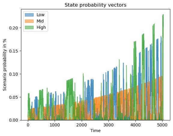
    imp_vol_state, np.percentile(imp_vol_state, [25, 75]), half_life=T / 2)
stationary_transformations_sim = ffr.simulate(S, H, probs, states)
For installation instructions, see the fortitudo.tech GitHub repo (give it a star if you want us to continue adding free functionality like this).
Note that if you want to generate very fast simulations and use multiple continuous or discrete state variables, you must subscribe to the Investment Simulation module.
Why we decided to add the functionality
First of all due to user requests but also because we don’t want to replicate the same lines of code in all of the open-source examples where we simulate future market paths like example 11 and example 13.
We will soon present new methods for analyzing fully general market paths. We are very excited to share them and think that they will be game changers. To make sure that you do not miss out on this, subscribe to the Quantamental Investing publication.
If you subscribe using your work email, consider expensing the subscription and potentially using the group subscription option to save 20% for you and your colleagues.
You can find all the paid content here. You might in particular be interested in the Applied Quantitative Investment Management course and the expanding collection of exclusive case studies.
You can watch the first lecture of the Applied Quantitative Investment Management course for free below:

