
Better Backtesting
This post introduces a backtesting approach that leverages synthetic market data to overcome the primary limitation of historical backtesting.

I recently wrote a post about naive backtesting of investment risk measures1, which is usually performed in the following way:
Look at some historical data samples.
Optimize portfolios using different risk measures.
Crown the investment risk measure with the highest cumulative performance as “the best investment risk measure”.
The above approach is usually performed by people who introduce a new investment risk measure and want to promote it.
However, the issue is that it is hard to justify making generalized conclusions based on one historical realization.
It is almost certain that if we chose a slightly different backtest configuration with different constraints or risk targets, then another investment risk measure would come out on top.
So, people usually just look for backtest configurations that fit the story that they want to tell.
It is the same approach that some people use to promote investment strategies to less sophisticated investors, who do not spot the problem.
For more perspectives on this naive backtesting approach, watch the end of the second lecture of the Applied Quantitative Investment Management course:
The essence of a good investment risk measure
As I argue in the Portfolio Construction and Risk Management book2, what determines a good investment risk measure should be determined by the following:
Focus on minimizing the risks that we want to avoid, i.e., large losses.
Is meaningful for fully general distributions.
Respects the diversification principle.
Is easy to interpret and understand.
When it comes to the variance risk measure, it fails in relation to point 1. and 2. (and in fact also point 4. for normal people).
Value-at-Risk (VaR) fails in relation to point 3., while Conditional Value-at-Risk (CVaR) satisfies them all.
There might be other more exotic tail risk measures but point 4. is essential for broad adoptability. Investment management clients and other nontechnical stakeholders simply must have some sense of what the investment risk measure means.
Hence, CVaR is the preferred tail risk measure among both market makers and investment managers, who are increasingly starting to discard variance.
For more perspectives, watch the video below:
A better backtesting procedure
As Section 3.6 in the Portfolio Construction and Risk Management book explains, the main issue with the historical backtesting procedure is that it uses just one historical path. Hence, it is very easy to overfit on this one historical path if we are not extremely careful.
It is also dangerous to make generalized conclusions based on one path, in the same way that it would be dangerous to draw the conclusion that we can only generate positive numbers from the normal distribution because our single realization happened to be positive.
While investment distributions are usually not estimated based on a single observation, but several observations over time and potentially of different, related risk factors and instruments, the one observation analogy for historical realizations of specific investment strategies is probably not too bad.
To improve the historical backtesting procedure, we want to be able to generate new joint paths for investment markets that have similar characteristics to the historical ones but give us different realizations that we can validate our investment strategies on.
While this might sound straightforward in theory, it is challenging and not perfect in practice, because we must be able to properly estimate a model for potentially high-dimensional market simulation of new paths.
In Section 3.6 of the Portfolio Construction and Risk Management book, we use the Fully Flexible Resampling method, which is an instance of the newly introduced Time- and State-Dependent Resampling3 class, to generate new paths for 10 US equity indices using VIX as the state variable and compare CVaR to variance optimization.
You can find all the details and perspectives in the Portfolio Construction and Risk Management book, including Python code that allows you to adjust the parameters of the backtest, and a video walkthrough at the end of the fourth lecture in the Applied Quantitative Investment Management course.
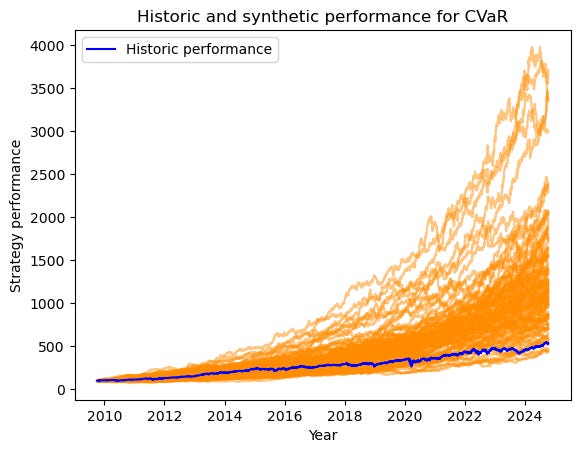
The cover image in this post shows the historical performance of the CVaR optimized portfolio in addition to 100 synthetic paths. While the historical performance falls into the range of simulated outcomes, it seems that the model calibration is a bit too optimistic. Hence, we can improve on that by using more state variables or careful time-conditioning.
An interesting result from the case study is perhaps that we only use S=100 simulations to compute the 90%-CVaR optimized portfolios, which leave us with just 10 observations below the 90%-VaR value.
Interestingly, the 10 observations are sufficient to result in CVaR optimized portfolios that have historically outperformed the variance optimized portfolios, see this Note:
Naive Backtesting post: https://antonvorobets.substack.com/p/naive-backtesting
Portfolio Construction and Risk Management Book post: https://antonvorobets.substack.com/p/pcrm-book
Time- and State-Dependent Resampling SSRN article: https://ssrn.com/abstract=5117589