Multi-Asset Macro Model

This article explains how the real rate, inflation, and growth factors can be defined in a multi-asset macro model, including a practical Python case study.

Visualization of joint macro factor conditioning for growth, inflation, and real rate.

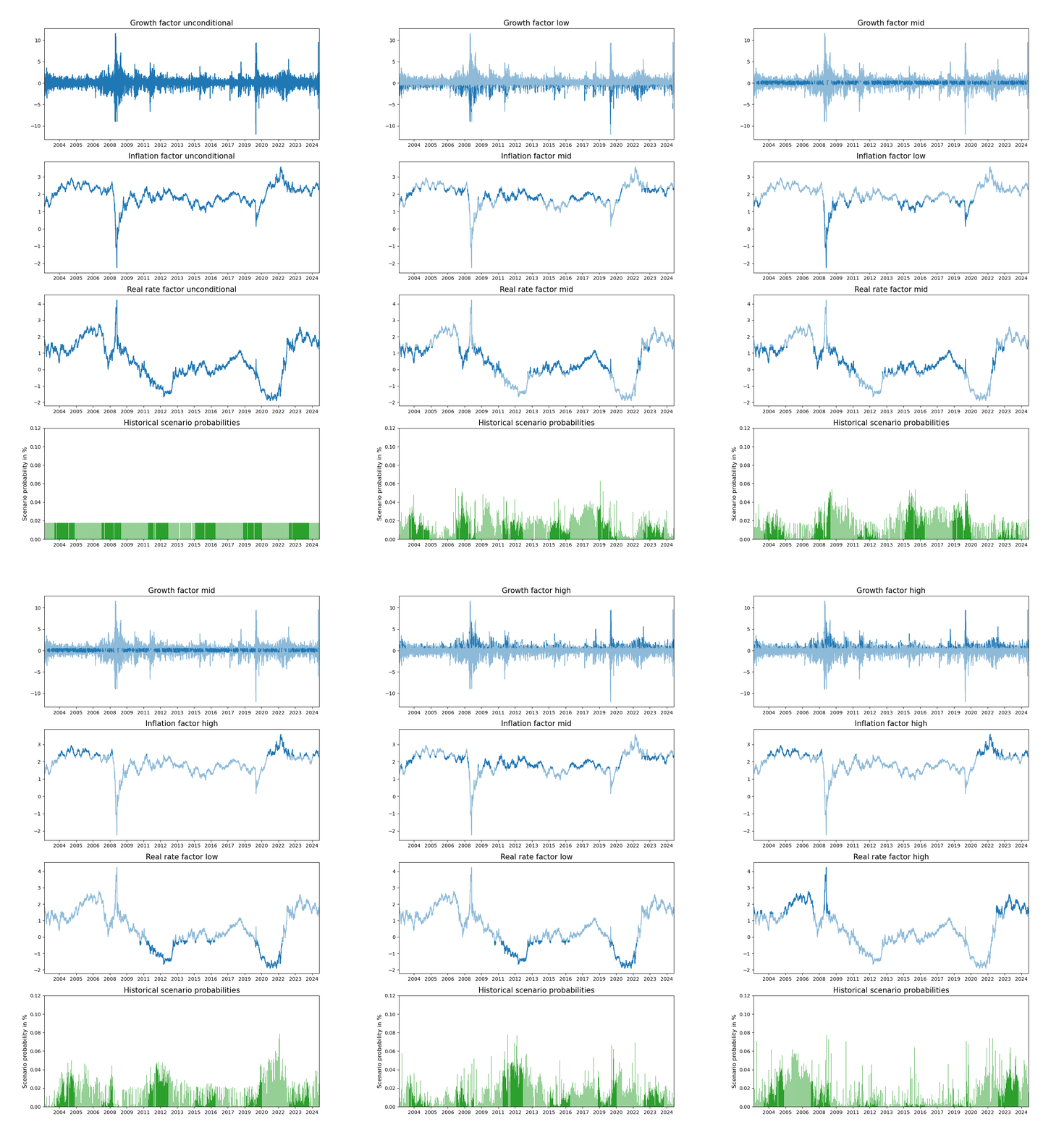
Examples that use the Causal and Predictive Market Views and Stress-Testing framework often show a Bayesian network with the three main factors being real rate, inflation, and growth.

The main idea is that we want to translate our hypotheses and views about the macroeconomy into investment P&L, watch this video for an explanation.

This is indeed often the perspective of the Chief Investment Officer (CIO), who is usually responsible for the overall exposure to both asset classes and broad risk factors, while intra-asset-class decisions are delegated to more focused investment managers.

For a deep and coherent presentation of the Causal and Predictive Market Views and Stress-Testing framework as well as the associated Sequential Entropy Pooling method, see the Portfolio Construction and Risk Management book.

Integration with the next generation investment framework

The next generation investment framework allows us to incorporate macro factors in a seamless way and even combine them with asset class specific factors such as value and growth for equities.

This follows from the fact that our investment market Monte Carlo simulations are collected into one matrix R given by:

\(R=\left(\begin{array}{cccc} R_{1,1} & R_{1,2} & \cdots & R_{1,I}\\ R_{2,1} & R_{2,2} & \cdots & R_{2,I}\\ \vdots & \vdots & \ddots & \vdots\\ R_{S,1} & R_{S,2} & \cdots & R_{S,I} \end{array}\right).\)

The columns of R represent marginal distribution simulations for return, risk factor, or macro factor i=1,2,…,I, while the rows of R represents the joint simulation scenarios for all the returns and factors.

Hence, we simply add columns with the macro factors in addition to the risk factors such as interest rates and implied volatilities that we use for pricing, see Chapter 4 in the Portfolio Construction and Risk Management book.

In this way, we have consistent joint scenarios for all the returns and factors that are relevant for our portfolios. We can then isolate specific scenarios for the factors both historically and in our simulation to analyze the effect on our portfolio returns.

This is the first case study in a monthly series of exclusive cases that use the next generation investment framework for real-world investment analysis. Find the other paid Quantamental Investing posts here.

Factor definition and Python case study