
Optimal Gold Allocation
This article performs CVaR portfolio optimization to assess the size of the optimal gold allocation for portfolios with various risk targets.

This case study continues where we left off in the Gold in Multi-Asset Portfolios case study, where we performed Fully Flexible Resampling (FFR) simulation using the Multi-Asset Macro Model and added several instantaneous stress tests to analyze gold’s properties on multiple horizons.
In this case study, we proceed to optimize the CVaR of portfolios with various risk targets to see what the optimal gold allocation is for different risk levels.
We also include some Sequential Entropy Pooling (SeqEP) views and stress testing for a more nuanced analysis.
For more details about all the above methods, you can read the Portfolio Construction and Risk Management book and complete the Applied Quantitative Investment Management course.
Python case study
To define multi-asset portfolios that are “low”, “medium”, and “high” risk, we use the same benchmarks as in the Tactical Asset Allocation Performance Lower Bound case study:
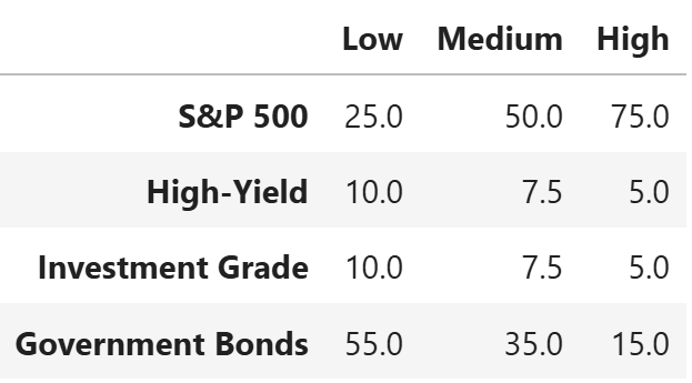
These portfolios give us CVaR risk targets that we can use for optimization, with and without a CVaR tracking error constraint.
For the nuances of the tracking error constraint, watch Lecture 9 on Portfolio Optimization in the Applied Quantitative Investment Management course.
Below, you will first see the one-year simulation statistics of the five ETFs that we used in the Gold in Multi-Asset Portfolios case study, i.e., IVV (S&P 500), HYG (US high-yield), LQD (US investment-grade), IEF (7-10y US government bonds), and GLD (gold).
We then continue to compute the CVaR of the three benchmark portfolios and optimize with these risk targets for the overall portfolio.
After that, we optimize with a 2% CVaR tracking error constraint to assess if the risk budget would be used for gold or not.
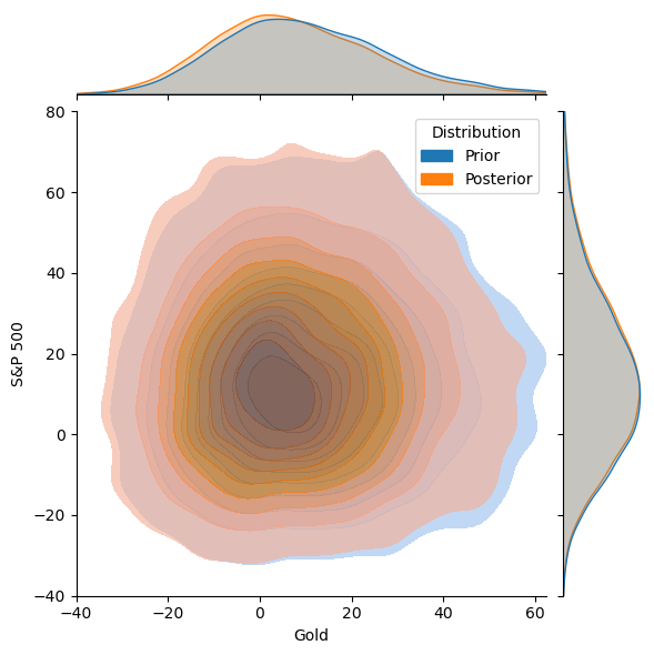
We repeat the above analysis for both the prior simulation and Sequential Entropy Pooling stress tests, where we purposefully make gold’s properties less attractive by reducing the expected return and increasing its CVaR.
The Python code that performs all these computations and uses the Investment Analysis module is available at the bottom of this post.
To keep this case study at a manageable length, we perform optimization without Resampled Portfolio Stacking parameter uncertainty, which you can learn more about in Lecture 10 about Resampled Portfolio Optimization.
We will introduce this uncertainty in future case studies and focus on the nuances of stacking objectives.
Base case optimization and risk results
The simulation from the Gold in Multi-Asset Portfolios case study produces the following prior statistics for the five ETFs on the yearly horizon: